上篇文章中我们讲解了卷积神经网络的基本原理,包括几个基本层的定义、运算规则等。本文主要写卷积神经网络如何进行一次完整的训练,包括前向传播和反向传播,并自己手写一个卷积神经网络。如果不了解基本原理的,可以先看看上篇文章:【深度学习系列】卷积神经网络CNN原理详解(一)——基本原理
卷积神经网络的前向传播
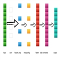
首先我们来看一个最简单的卷积神经网络:
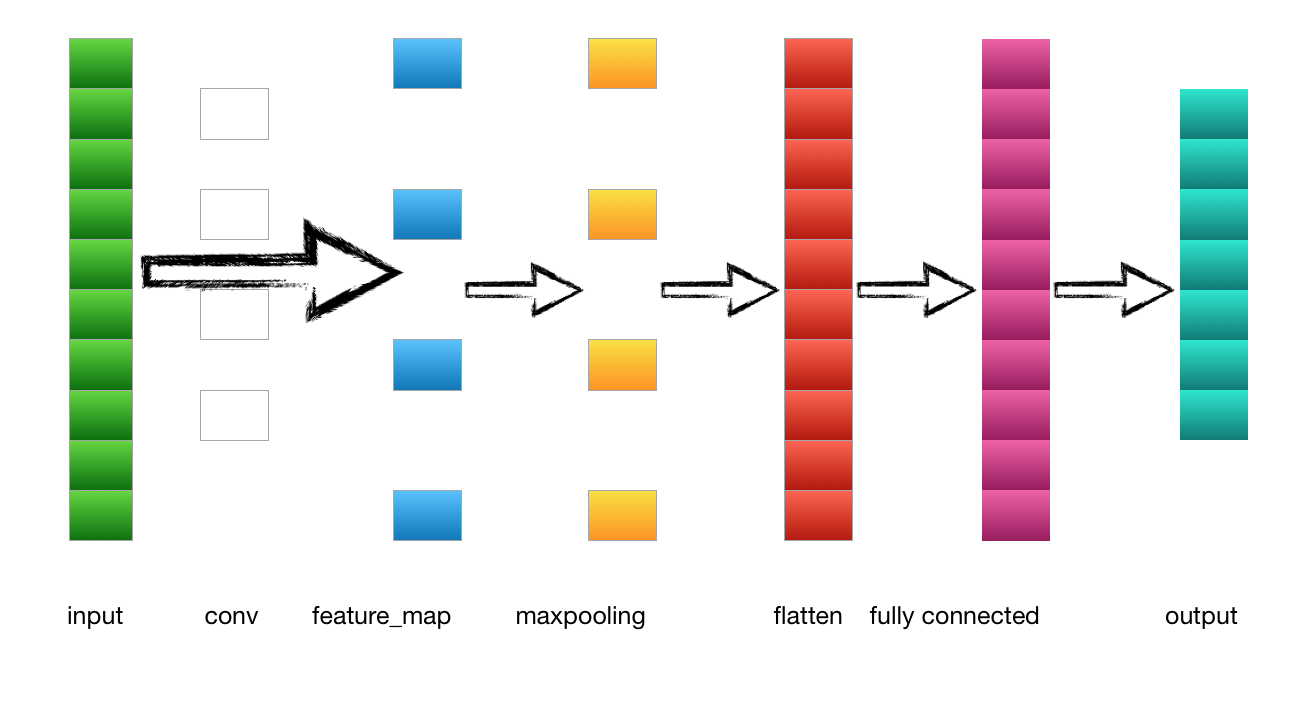
1.输入层---->卷积层
以上一节的例子为例,输入是一个4*4 的image,经过两个2*2的卷积核进行卷积运算后,变成两个3*3的feature_map
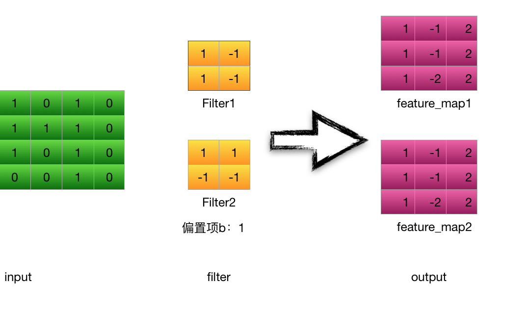
以卷积核filter1为例(stride = 1 ):
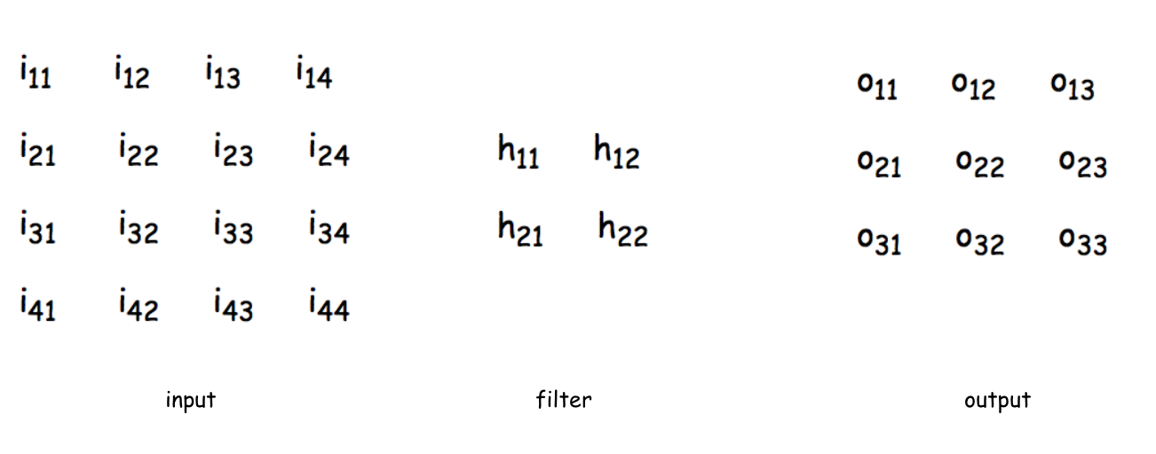
计算第一个卷积层神经元o11的输入:
\begin{equation}
\begin{aligned}
\ net_{o_{11}}&= conv (input,filter)\\
&= i_{11} \times h_{11} + i_{12} \times h_{12} +i_{21} \times h_{21} + i_{22} \times h_{22}\\
&=1 \times 1 + 0 \times (-1) +1 \times 1 + 1 \times (-1)=1
\end{aligned}
\end{equation}
神经元o11的输出:(此处使用Relu激活函数)
\begin{equation}
\begin{aligned}
out_{o_{11}} &= activators(net_{o_{11}}) \\
&=max(0,net_{o_{11}}) = 1
\end{aligned}
\end{equation}
其他神经元计算方式相同
2.卷积层---->池化层
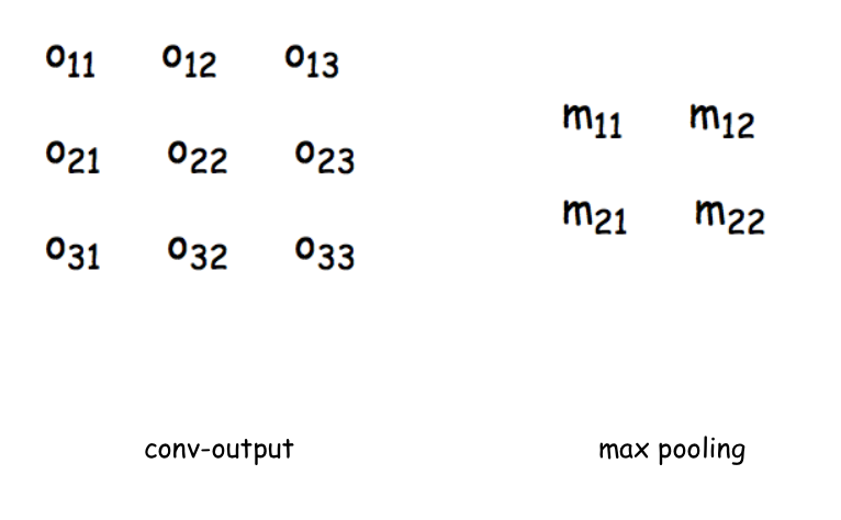
计算池化层m11 的输入(取窗口为 2 * 2),池化层没有激活函数
\begin{equation}
\begin{aligned}
net_{m_{11}} &= max(o_{11},o_{12},o_{21},o_{23}) = 1\\
&out_{m_{11}} = net_{m_{11}} = 1
\end{aligned}
\end{equation}
3.池化层---->全连接层
池化层的输出到flatten层把所有元素“拍平”,然后到全连接层。
4.全连接层---->输出层
全连接层到输出层就是正常的神经元与神经元之间的邻接相连,通过softmax函数计算后输出到output,得到不同类别的概率值,输出概率值最大的即为该图片的类别。
卷积神经网络的反向传播
传统的神经网络是全连接形式的,如果进行反向传播,只需要由下一层对前一层不断的求偏导,即求链式偏导就可以求出每一层的误差敏感项,然后求出权重和偏置项的梯度,即可更新权重。而卷积神经网络有两个特殊的层:卷积层和池化层。池化层输出时不需要经过激活函数,是一个滑动窗口的最大值,一个常数,那么它的偏导是1。池化层相当于对上层图片做了一个压缩,这个反向求误差敏感项时与传统的反向传播方式不同。从卷积后的feature_map反向传播到前一层时,由于前向传播时是通过卷积核做卷积运算得到的feature_map,所以反向传播与传统的也不一样,需要更新卷积核的参数。下面我们介绍一下池化层和卷积层是如何做反向传播的。
在介绍之前,首先回顾一下传统的反向传播方法:
1.通过前向传播计算每一层的输入值$net_{i,j}$ (如卷积后的feature_map的第一个神经元的输入:neto11)
2.反向传播计算每个神经元的误差项$\delta_{i,j}$ ,$\delta_{i,j} = \frac{\partial E}{\partial net_{i,j}}$,其中E为损失函数计算得到的总体误差,可以用平方差,交叉熵等表示。
3.计算每个神经元权重$w_{i,j}$ 的梯度,$\eta_{i,j} = \frac{\partial E}{\partial net_{i,j}} \cdot \frac{\partial net_{i,j}}{\partial w_{i,j}} = \delta_{i,j} \cdot a_i$
4.更新权重 $w_{i,j} = w_{i,j}-\lambda \cdot \eta_{i,j}$(其中$\lambda$为学习率)
卷积层的反向传播
由前向传播可得:
\begin{equation}
\begin{aligned}
\ net_{o_{11}}&= conv (input,filter)\\
&= i_{11} \times h_{11} + i_{12} \times h_{12} +i_{21} \times h_{21} + i_{22} \times h_{22}\\
out_{o_{11}} &= activators(net_{o_{11}}) \\
&=max(0,net_{o_{11}})
\end{aligned}
\end{equation}
首先计算输入层的误差项$\delta_{11}$
$$\delta_{11} = \frac{\partial E}{\partial net_{o_{11}}} =\frac{\partial E}{\partial out_{o_{11}}} \cdot \frac{\partial out_{o_{11}}}{\partial net_{o_{11}}}$$
先计算$\frac{\partial E}{\partial out_{o_{11}}}$
$i_{11}$的偏导:
\begin{equation}
\begin{aligned}
\because net_{o_{11}}&= conv (input,filter)\\
&= i_{11} \times h_{11} + i_{12} \times h_{12} +i_{21} \times h_{21} + i_{22} \times h_{22}\\
\therefore \frac{\partial E}{\partial i_{11}}&=\frac{\partial E}{\partial net_{o_{11}}} \cdot \frac{\partial net_{o_{11}}}{\partial i_{11}}\\
&=\delta_{11} \cdot h_{11}
\end{aligned}
\end{equation}
$i_{12}$的偏导:
\begin{equation}
\begin{aligned}
\because net_{o_{11}}&= conv (input,filter)\\
&= i_{11} \times h_{11} + i_{12} \times h_{12} +i_{21} \times h_{21} + i_{22} \times h_{22}\\
net_{o_{12}}&= conv (input,filter)\\
&= i_{12} \times h_{11} + i_{13} \times h_{12} +i_{22} \times h_{21} + i_{23} \times h_{22}\\
\therefore \frac{\partial E}{\partial i_{12}}&=\frac{\partial E}{\partial net_{o_{11}}} \cdot \frac{\partial net_{o_{11}}}{\partial i_{12}} +\frac{\partial E}{\partial net_{o_{12}}} \cdot \frac{\partial net_{o_{12}}}{\partial i_{12}}\\
&=\delta_{11} \cdot h_{12}+\delta_{12} \cdot h_{11}
\end{aligned}
\end{equation}
$i_{22}的偏导$:
\begin{equation}
\begin{aligned}
\because &i_{21}与net_{o_{11}}、net_{o_{12}}、net_{o_{21}}、net_{o_{22}}有关\\
\therefore
\frac{\partial E}{\partial i_{22}}&=\frac{\partial E}{\partial net_{o_{11}}} \cdot \frac{\partial net_{o_{11}}}{\partial i_{22}} +\frac{\partial E}{\partial net_{o_{12}}} \cdot \frac{\partial net_{o_{12}}}{\partial i_{22}}\\
&+\frac{\partial E}{\partial net_{o_{21}}} \cdot \frac{\partial net_{o_{21}}}{\partial i_{22}}+\frac{\partial E}{\partial net_{o_{22}}} \cdot \frac{\partial net_{o_{22}}}{\partial i_{22}}\\
&=\delta_{11} \cdot h_{22}+\delta_{12} \cdot h_{21}+\delta_{21} \cdot h_{12}+\delta_{22} \cdot h_{11}
\end{aligned}
\end{equation}
观察以上几个式子可以得出,想要计算误差敏感项${\delta_{i,j}},即$$\frac{\partial E}{\partial net_{o_{11}}}$,相当于就是把这个误差敏感矩阵的周围补了一圈零,与进行180°翻转后的卷积核filter进行卷积运算,则可以计算
$$\frac{\partial E}{\partial out_{i,j}} = \sum_m \cdot \sum_n h_{m,n}\delta_{i+m,j+n}$$
此时我们的误差敏感矩阵就求完了,得到误差敏感矩阵后,即可求权重的梯度
权重的梯度:
\begin{equation}
\begin{aligned}
\frac{\partial E}{\partial w_{i,j}} = \sum_m\sum_n\delta_{m,n}out_{o_{i+m,j+n}}
\end{aligned}
\end{equation}
误差项的梯度:
\begin{equation}
\begin{aligned}
\because out_{o_{11}} &= activators(net_{o_{11}})\\
&=f'(net_{o_{11}})\\
\therefore \delta_{i_{11}} &=\frac{\partial E}{\partial net_{o_{11}}} \\
&=\frac{\partial E}{\partial out_{o_{11}}} \cdot \frac{\partial out_{o_{11}}}{\partial net_{o_{11}}}\\
&=\sum_m \cdot \sum_n h_{m,n}\delta_{i+m,j+n} \cdot f'(net_{o_{11}})
\end{aligned}
\end{equation}
得到了权重和偏置项的梯度后,就可以根据梯度下降法更新权重和梯度了。
池化层的反向传播
公式太多了,留个坑,等会再写
手写一个卷积神经网络
1.定义一个卷积层
首先我们通过ConvLayer来实现一个卷积层,定义卷积层的超参数
 1 class ConvLayer(object):
 2     '''
 3     参数含义:
 4     input_width:输入图片尺寸——宽度
 5     input_height:输入图片尺寸——长度
 6     channel_number:通道数,彩色为3,灰色为1
 7     filter_width:卷积核的宽
 8     filter_height:卷积核的长
 9     filter_number:卷积核数量
10     zero_padding:补零长度
11     stride:步长
12     activator:激活函数
13     learning_rate:学习率
14     '''
15     def __init__(self, input_width, input_height,
16                  channel_number, filter_width,
17                  filter_height, filter_number,
18                  zero_padding, stride, activator,
19                  learning_rate):
20         self.input_width = input_width
21         self.input_height = input_height
22         self.channel_number = channel_number
23         self.filter_width = filter_width
24         self.filter_height = filter_height
25         self.filter_number = filter_number
26         self.zero_padding = zero_padding
27         self.stride = stride
28         self.output_width = \
29             ConvLayer.calculate_output_size(
30             self.input_width, filter_width, zero_padding,
31             stride)
32         self.output_height = \
33             ConvLayer.calculate_output_size(
34             self.input_height, filter_height, zero_padding,
35             stride)
36         self.output_array = np.zeros((self.filter_number,
37             self.output_height, self.output_width))
38         self.filters = []
39         for i in range(filter_number):
40             self.filters.append(Filter(filter_width,
41                 filter_height, self.channel_number))
42         self.activator = activator
43         self.learning_rate = learning_rate
其中calculate_output_size用来计算通过卷积运算后输出的feature_map大小
1 @staticmethod
2     def calculate_output_size(input_size,
3             filter_size, zero_padding, stride):
4         return (input_size - filter_size +
5             2 * zero_padding) / stride + 1
2.构造一个激活函数
此处用的是RELU激活函数,因此我们在activators.py里定义,forward是前向计算,backforward是计算公式的导数:
1 class ReluActivator(object):
2     def forward(self, weighted_input):
3         #return weighted_input
4         return max(0, weighted_input)
5
6     def backward(self, output):
7         return 1 if output > 0 else 0
其他常见的激活函数我们也可以放到activators里,如sigmoid函数,我们可以做如下定义:
1 class SigmoidActivator(object):
2     def forward(self, weighted_input):
3         return 1.0 / (1.0 + np.exp(-weighted_input))
4     #the partial of sigmoid
5     def backward(self, output):
6         return output * (1 - output)
如果我们需要自动以其他的激活函数,都可以在activator.py定义一个类即可。
3.定义一个类,保存卷积层的参数和梯度
 1 class Filter(object):
 2     def __init__(self, width, height, depth):
 3         #初始权重
 4         self.weights = np.random.uniform(-1e-4, 1e-4,
 5             (depth, height, width))
 6         #初始偏置
 7         self.bias = 0
 8         self.weights_grad = np.zeros(
 9             self.weights.shape)
10         self.bias_grad = 0
11
12     def __repr__(self):
13         return 'filter weights:\n%s\nbias:\n%s' % (
14             repr(self.weights), repr(self.bias))
15
16     def get_weights(self):
17         return self.weights
18
19     def get_bias(self):
20         return self.bias
21
22     def update(self, learning_rate):
23         self.weights -= learning_rate * self.weights_grad
24         self.bias -= learning_rate * self.bias_grad
4.卷积层的前向传播
1).获取卷积区域
 1 # 获取卷积区域
 2 def get_patch(input_array, i, j, filter_width,
 3               filter_height, stride):
 4     '''
 5     从输入数组中获取本次卷积的区域,
 6     自动适配输入为2D和3D的情况
 7     '''
 8     start_i = i * stride
 9     start_j = j * stride
10     if input_array.ndim == 2:
11         input_array_conv = input_array[
12             start_i : start_i + filter_height,
13             start_j : start_j + filter_width]
14         print "input_array_conv:",input_array_conv
15         return input_array_conv
16
17     elif input_array.ndim == 3:
18         input_array_conv = input_array[:,
19             start_i : start_i + filter_height,
20             start_j : start_j + filter_width]
21         print "input_array_conv:",input_array_conv
22         return input_array_conv
2).进行卷积运算
 1 def conv(input_array,
 2          kernel_array,
 3          output_array,
 4          stride, bias):
 5     '''
 6     计算卷积,自动适配输入为2D和3D的情况
 7     '''
 8     channel_number = input_array.ndim
 9     output_width = output_array.shape[1]
10     output_height = output_array.shape[0]
11     kernel_width = kernel_array.shape[-1]
12     kernel_height = kernel_array.shape[-2]
13     for i in range(output_height):
14         for j in range(output_width):
15             output_array[i][j] = (
16                 get_patch(input_array, i, j, kernel_width,
17                     kernel_height, stride) * kernel_array
18                 ).sum() + bias
3).增加zero_padding
 1 #增加Zero padding
 2 def padding(input_array, zp):
 3     '''
 4     为数组增加Zero padding,自动适配输入为2D和3D的情况
 5     '''
 6     if zp == 0:
 7         return input_array
 8     else:
 9         if input_array.ndim == 3:
10             input_width = input_array.shape[2]
11             input_height = input_array.shape[1]
12             input_depth = input_array.shape[0]
13             padded_array = np.zeros((
14                 input_depth,
15                 input_height + 2 * zp,
16                 input_width + 2 * zp))
17             padded_array[:,
18                 zp : zp + input_height,
19                 zp : zp + input_width] = input_array
20             return padded_array
21         elif input_array.ndim == 2:
22             input_width = input_array.shape[1]
23             input_height = input_array.shape[0]
24             padded_array = np.zeros((
25                 input_height + 2 * zp,
26                 input_width + 2 * zp))
27             padded_array[zp : zp + input_height,
28                 zp : zp + input_width] = input_array
29             return padded_array
4).进行前向传播
 1 def forward(self, input_array):
 2         '''
 3         计算卷积层的输出
 4         输出结果保存在self.output_array
 5         '''
 6         self.input_array = input_array
 7         self.padded_input_array = padding(input_array,
 8             self.zero_padding)
 9         for f in range(self.filter_number):
10             filter = self.filters[f]
11             conv(self.padded_input_array,
12                 filter.get_weights(), self.output_array[f],
13                 self.stride, filter.get_bias())
14         element_wise_op(self.output_array,
15                         self.activator.forward)
其中element_wise_op函数是将每个组的元素对应相乘
1 # 对numpy数组进行element wise操作,将矩阵中的每个元素对应相乘
2 def element_wise_op(array, op):
3     for i in np.nditer(array,
4                        op_flags=['readwrite']):
5         i[...] = op(i)
5.卷积层的反向传播
1).将误差传递到上一层
 1 def bp_sensitivity_map(self, sensitivity_array,
 2                            activator):
 3         '''
 4         计算传递到上一层的sensitivity map
 5         sensitivity_array: 本层的sensitivity map
 6         activator: 上一层的激活函数
 7         '''
 8         # 处理卷积步长,对原始sensitivity map进行扩展
 9         expanded_array = self.expand_sensitivity_map(
10             sensitivity_array)
11         # full卷积,对sensitivitiy map进行zero padding
12         # 虽然原始输入的zero padding单元也会获得残差
13         # 但这个残差不需要继续向上传递,因此就不计算了
14         expanded_width = expanded_array.shape[2]
15         zp = (self.input_width +
16               self.filter_width - 1 - expanded_width) / 2
17         padded_array = padding(expanded_array, zp)
18         # 初始化delta_array,用于保存传递到上一层的
19         # sensitivity map
20         self.delta_array = self.create_delta_array()
21         # 对于具有多个filter的卷积层来说,最终传递到上一层的
22         # sensitivity map相当于所有的filter的
23         # sensitivity map之和
24         for f in range(self.filter_number):
25             filter = self.filters[f]
26             # 将filter权重翻转180度
27             flipped_weights = np.array(map(
28                 lambda i: np.rot90(i, 2),
29                 filter.get_weights()))
30             # 计算与一个filter对应的delta_array
31             delta_array = self.create_delta_array()
32             for d in range(delta_array.shape[0]):
33                 conv(padded_array[f], flipped_weights[d],
34                     delta_array[d], 1, 0)
35             self.delta_array += delta_array
36         # 将计算结果与激活函数的偏导数做element-wise乘法操作
37         derivative_array = np.array(self.input_array)
38         element_wise_op(derivative_array,
39                         activator.backward)
40         self.delta_array *= derivative_array
2).保存传递到上一层的sensitivity map的数组
1 def create_delta_array(self):
2         return np.zeros((self.channel_number,
3             self.input_height, self.input_width))
3).计算代码梯度
 1 def bp_gradient(self, sensitivity_array):
 2         # 处理卷积步长,对原始sensitivity map进行扩展
 3         expanded_array = self.expand_sensitivity_map(
 4             sensitivity_array)
 5         for f in range(self.filter_number):
 6             # 计算每个权重的梯度
 7             filter = self.filters[f]
 8             for d in range(filter.weights.shape[0]):
 9                 conv(self.padded_input_array[d],
10                      expanded_array[f],
11                      filter.weights_grad[d], 1, 0)
12             # 计算偏置项的梯度
13             filter.bias_grad = expanded_array[f].sum()
4).按照梯度下降法更新参数
1 def update(self):
2         '''
3         按照梯度下降,更新权重
4         '''
5         for filter in self.filters:
6             filter.update(self.learning_rate)
6.MaxPooling层的训练
1).定义MaxPooling类
 1 class MaxPoolingLayer(object):
 2     def __init__(self, input_width, input_height,
 3                  channel_number, filter_width,
 4                  filter_height, stride):
 5         self.input_width = input_width
 6         self.input_height = input_height
 7         self.channel_number = channel_number
 8         self.filter_width = filter_width
 9         self.filter_height = filter_height
10         self.stride = stride
11         self.output_width = (input_width -
12             filter_width) / self.stride + 1
13         self.output_height = (input_height -
14             filter_height) / self.stride + 1
15         self.output_array = np.zeros((self.channel_number,
16             self.output_height, self.output_width))
2).前向传播计算
 1 # 前向传播
 2     def forward(self, input_array):
 3         for d in range(self.channel_number):
 4             for i in range(self.output_height):
 5                 for j in range(self.output_width):
 6                     self.output_array[d,i,j] = (
 7                         get_patch(input_array[d], i, j,
 8                             self.filter_width,
 9                             self.filter_height,
10                             self.stride).max())
3).反向传播计算
 1 #反向传播
 2     def backward(self, input_array, sensitivity_array):
 3         self.delta_array = np.zeros(input_array.shape)
 4         for d in range(self.channel_number):
 5             for i in range(self.output_height):
 6                 for j in range(self.output_width):
 7                     patch_array = get_patch(
 8                         input_array[d], i, j,
 9                         self.filter_width,
10                         self.filter_height,
11                         self.stride)
12                     k, l = get_max_index(patch_array)
13                     self.delta_array[d,
14                         i * self.stride + k,
15                         j * self.stride + l] = \
16                         sensitivity_array[d,i,j]
完整代码请见:cnn.py (https://github.com/huxiaoman7/PaddlePaddle_code/blob/master/1.mnist/cnn.py)
最后,我们用之前的4 * 4的image数据检验一下通过一次卷积神经网络进行前向传播和反向传播后的输出结果:
 1 def init_test():
 2     a = np.array(
 3         [[[0,1,1,0,2],
 4           [2,2,2,2,1],
 5           [1,0,0,2,0],
 6           [0,1,1,0,0],
 7           [1,2,0,0,2]],
 8          [[1,0,2,2,0],
 9           [0,0,0,2,0],
10           [1,2,1,2,1],
11           [1,0,0,0,0],
12           [1,2,1,1,1]],
13          [[2,1,2,0,0],
14           [1,0,0,1,0],
15           [0,2,1,0,1],
16           [0,1,2,2,2],
17           [2,1,0,0,1]]])
18     b = np.array(
19         [[[0,1,1],
20           [2,2,2],
21           [1,0,0]],
22          [[1,0,2],
23           [0,0,0],
24           [1,2,1]]])
25     cl = ConvLayer(5,5,3,3,3,2,1,2,IdentityActivator(),0.001)
26     cl.filters[0].weights = np.array(
27         [[[-1,1,0],
28           [0,1,0],
29           [0,1,1]],
30          [[-1,-1,0],
31           [0,0,0],
32           [0,-1,0]],
33          [[0,0,-1],
34           [0,1,0],
35           [1,-1,-1]]], dtype=np.float64)
36     cl.filters[0].bias=1
37     cl.filters[1].weights = np.array(
38         [[[1,1,-1],
39           [-1,-1,1],
40           [0,-1,1]],
41          [[0,1,0],
42          [-1,0,-1],
43           [-1,1,0]],
44          [[-1,0,0],
45           [-1,0,1],
46           [-1,0,0]]], dtype=np.float64)
47     return a, b, cl
运行一下:
 1 def test():
 2     a, b, cl = init_test()
 3     cl.forward(a)
 4     print "前向传播结果:", cl.output_array
 5     cl.backward(a, b, IdentityActivator())
 6     cl.update()
 7     print "反向传播后更新得到的filter1:",cl.filters[0]
 8     print "反向传播后更新得到的filter2:",cl.filters[1]
 9
10 if __name__ == "__main__":
11         test()
运行结果:
 1 前向传播结果: [[[ 6.  7.  5.]
 2   [ 3. -1. -1.]
 3   [ 2. -1.  4.]]
 4
 5  [[ 2. -5. -8.]
 6   [ 1. -4. -4.]
 7   [ 0. -5. -5.]]]
 8 反向传播后更新得到的filter1: filter weights:
 9 array([[[-1.008,  0.99 , -0.009],
10         [-0.005,  0.994, -0.006],
11         [-0.006,  0.995,  0.996]],
12
13        [[-1.004, -1.001, -0.004],
14         [-0.01 , -0.009, -0.012],
15         [-0.002, -1.002, -0.002]],
16
17        [[-0.002, -0.002, -1.003],
18         [-0.005,  0.992, -0.005],
19         [ 0.993, -1.008, -1.007]]])
20 bias:
21 0.99099999999999999
22 反向传播后更新得到的filter2: filter weights:
23 array([[[  9.98000000e-01,   9.98000000e-01,  -1.00100000e+00],
24         [ -1.00400000e+00,  -1.00700000e+00,   9.97000000e-01],
25         [ -4.00000000e-03,  -1.00400000e+00,   9.98000000e-01]],
26
27        [[  0.00000000e+00,   9.99000000e-01,   0.00000000e+00],
28         [ -1.00900000e+00,  -5.00000000e-03,  -1.00400000e+00],
29         [ -1.00400000e+00,   1.00000000e+00,   0.00000000e+00]],
30
31        [[ -1.00400000e+00,  -6.00000000e-03,  -5.00000000e-03],
32         [ -1.00200000e+00,  -5.00000000e-03,   9.98000000e-01],
33         [ -1.00200000e+00,  -1.00000000e-03,   0.00000000e+00]]])
34 bias:
35 -0.0070000000000000001
总结
本文主要讲解了卷积神经网络中反向传播的一些技巧,包括卷积层和池化层的反向传播与传统的反向传播的区别,并实现了一个完整的CNN,后续大家可以自己修改一些代码,譬如当水平滑动长度与垂直滑动长度不同时需要怎么调整等等。如果有问题欢迎留言:)
参考文章:
1.https://www.cnblogs.com/pinard/p/6494810.html
2.https://www.zybuluo.com/hanbingtao/note/476663